3.19 Example: doping
The following example has been adapted from Nic Daéid et al. (2020).
A test designed to detect athletes who are doping is claimed to be ‘95% accurate.’ If an athlete is doping then the test returns positive 95% of the time, and if the athlete is not doping then the test returns negative 95% of the time. It is suspected that around 1 in every 50 athletes dope. An athlete tests positive for doping using this test during a random drugs screening. How likely is it that they are really doping?
Technical diagnostic testing information often needs to be `translated’ before it can be depicted clearly using a graphical representation. We can convert some of the above written information into the technical definitions. The second sentence states that the sensitivity and specificity are both 0.95, although the terms are not explicitly used. The base rate for doping is given as approximately 0.02.
Assume, for clarity, that we have a relevant population of 10,000 athletes. The technical information means the following:
- doping base rate: 0.02
- meaning: we expect 200 athletes to be doping and 9,800 not to be doping.
- test sensitivity: 0.95
- meaning: out of the expected 200 athletes who are doping, the test is expected to return positive for 190 of them and negative for 10 of them. We expect 10 false negatives.
- test specificity: 0.95
- meaning: out of the expected 9,800 athletes who are not doping, we expect 9,310 to test negative and 490 to test positive. We expect 490 false positives.
This is shown in the tree diagram format in Figure 3.6.
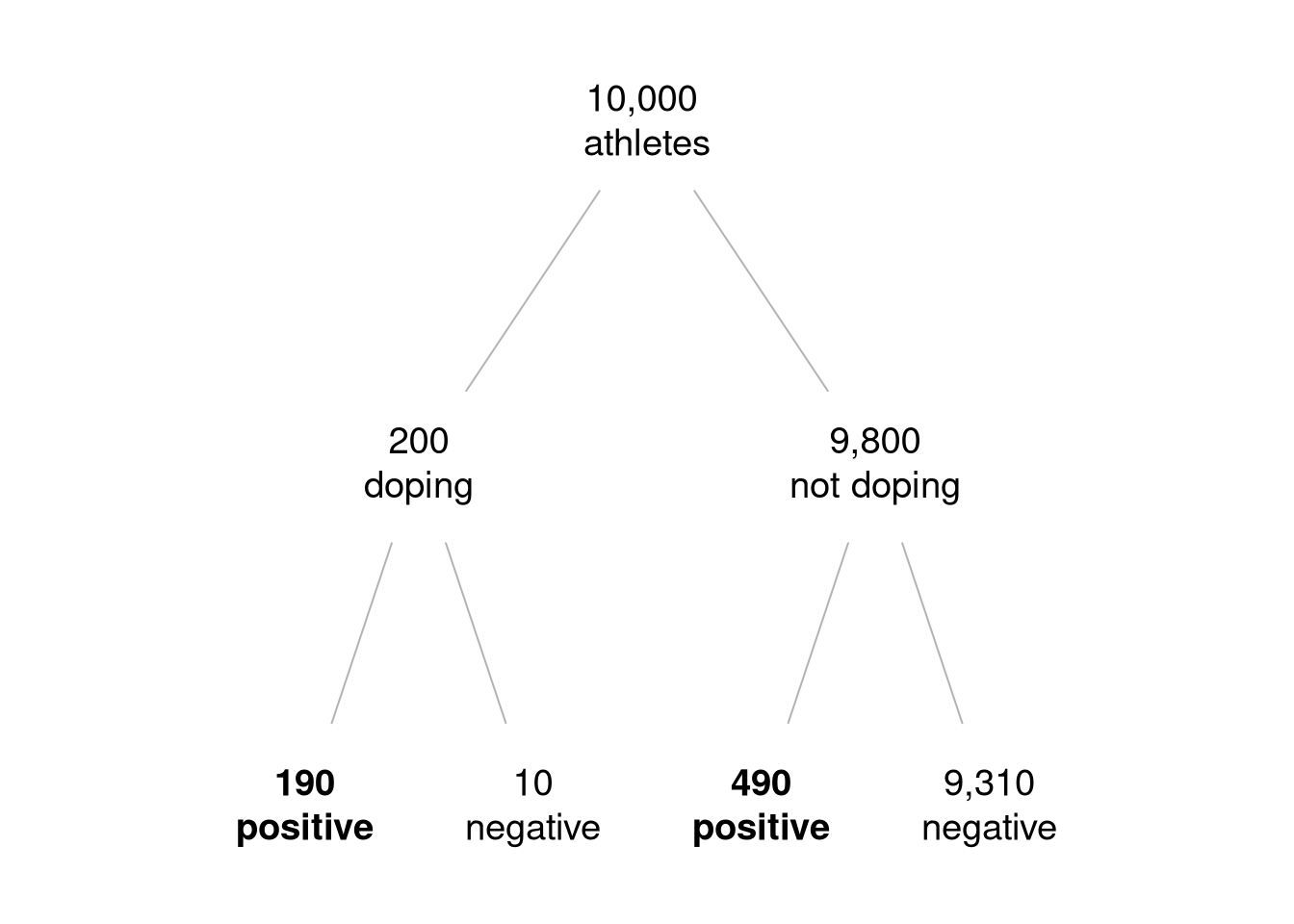
Figure 3.6: An expected frequency tree diagram of the doping example. Out of the 680 athletes who test positive (shown in bold font), 190 (~28%) are doping.
The answer to the question is that given a positive test result, we expect the athlete to be doping roughly 28% of the time. This is another example of how a low base rate can result in a low posterior probability, even when the testing error is relatively low.